Flint Water Crisis
Kettering University, Flint, MI
- Kettering University is a private institution that specializes in cooperative education. Through this pragmatic and experiential learning-based approach, being able to apply the knowledge gained in the classroom to solve real-world issues is what Kettering students do best, and when the Flint Water Crisis hit the city, the university rapidly became involved in a number of ways.
- Many served the community as volunteers, while proactive faculty created opportunities for students to learn from the effects of the crisis and give back in the process. With support from Professor Ghazi-Nezami, this project was provided an additional opportunity through MATH 327 (Mathematical Statistics), taught by Professor Boyan Dimitrov.
- The analysis is focused on water samples gathered from households.
Part A - Identifying Zip Codes

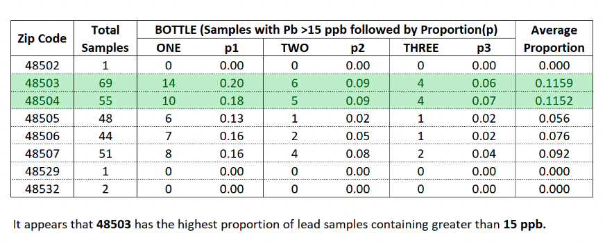
- This involved finding those zip codes with a sample proportion of lead over 15 parts per billion (ppb) and dividing them by the total number of samples to obtain a proportion.
- Columns 'ONE', 'TWO', and 'THREE' are the number of samples with a lead content greater than or equal to 15 ppb.
- Columns 'p1', 'p2', and 'p3' equate to the samples with lead content >= 15 ppb divided by the total number of samples.
- 48503 covers the area just around downtown Flint.
Part B — Normality Tests (statistical)
        ### IMPORTING REQUIRED PACKAGES ###
        import pandas as pd
        import numpy as np
        from matplotlib import pyplot as plt
        import seaborn as sns
        import scipy.stats as stats
        from statsmodels.graphics.gofplots import qqplot
        from statsmodels.stats.multicomp import pairwise_tukeyhsd
        from statsmodels.formula.api import ols

        ### UPLOADING CSV DATA TO DATAFRAME ###
        df_zip = pd.read_csv(r".\Dataset1.csv", encoding = "UTF-8")

        df_zip['Mean'] = df_zip[['Pb Bottle 1 (ppb) - First Draw',
            'Pb Bottle 2 (ppb) - 45 secs flushed',
            'Pb Bottle 3 (ppb) - 2 mins flushed']].mean(axis = 1)

            ### NORMALITY TESTS ###

            mn = [] #the mean of the zip code
            sd = [] #the standard deviation of the zip code
            length = [] #the number of samples in that zip code
            mv = [] #the highest lead content value for that zip code

            #test results
            shap = []
            da = []
            ad = []

            #p-values
            shapp = []
            dap = []

            #test-statistic
            shapst = []
            dast = []
            adst = []

            zipcodes = [48503, 48504, 48505, 48506, 48507]
            transformations = [2, 1, 0.5, 0, -.5, -1]
            zipcodes2 = []
            trnfrm = []

            for zipcode in zipcodes:
                cl = df_zip.loc[df_zip['Zip Code'] == zipcode, 'Mean']
                for i in transformations:
                    zipcodes2.append(zipcode)
                    trnfrm.append(i)
                    mn.append(np.mean(cl))
                    sd.append(np.std(cl))
                    length.append(len(cl))
                    mv.append(cl.max())

                    ## Transforming Data ##
                    bxcx = stats.boxcox(cl, i)

                    ##Shapiro
                    stat, p = stats.shapiro(bxcx)
                    shapst.append(stat)
                    shapp.append(p)
                    alpha = 0.05
                    if p > alpha:
                        shap.append('Sample looks Gaussian (fail to reject H0)')
                    else:
                        shap.append('Sample does not look Gaussian (reject H0)')

                    ##D'Agostino
                    stat, p = stats.normaltest(bxcx)
                    dast.append(stat)
                    dap.append(p)
                    alpha = 0.05
                    if p > alpha:
                        da.append('Sample looks Gaussian (fail to reject H0)')
                    else:
                        da.append('Sample does not look Gaussian (reject H0)')

                    ##AndersonDarling
                    statad = stats.anderson(bxcx)
                    p = 0
                    sl = statad.significance_level[2]
                    cv = statad.critical_values[2]
                    adst.append(statad.statistic)
                    if statad.statistic < statad.critical_values[2]:
                        ad.append('%.3f: %.3f, data looks normal (fail to reject H0)' % (sl, cv))
                    else:
                        ad.append('%.3f: %.3f, data does not look normal (reject H0)' % (sl, cv))


            results = pd.DataFrame({'Zipcodes':zipcodes2,
                                   'Indices':trnfrm,
                                   'Mean':mn,
                                   'Standard Deviation':sd,
                                   'Length':length,
                                   'Max':mv,
                                   'Shapiro Statistic':shapst,
                                   'Shapiro P-Value':shapp,
                                   'Shapiro result':shap,
                                   'DAgostino Statistic':dast,
                                   'DAgostino P-Value':dap,
                                   'DAgostino result':da,
                                   'AndersonDarling Statistic':adst,
                                   'AndersonDarling result':ad})

            #saving results to file
            rfile = results.to_csv(R"./NormalityTests.csv")
| Zipcodes |
Transformation |
Mean |
Standard Deviation |
Length |
Max |
Shapiro Statistic |
Shapiro P-Value |
Shapiro result |
DAgostino Statistic |
DAgostino P-Value |
DAgostino result |
AndersonDarling Statistic |
AndersonDarling result |
| 48503 |
0 |
6.793922705 |
9.358658096 |
69 |
40.89133333 |
0.963492632 |
0.041471705 |
Sample does not look Gaussian (reject H0) |
6.921262473 |
0.031409929 |
Sample does not look Gaussian (reject H0) |
0.616217481 |
5.000: 0.748, data looks normal (fail to reject H0) |
| 48504 |
0 |
16.96929091 |
52.35225346 |
55 |
353.1906667 |
0.906652749 |
0.000427611 |
Sample does not look Gaussian (reject H0) |
11.64674255 |
0.002957617 |
Sample does not look Gaussian (reject H0) |
1.821949035 |
5.000: 0.739, data does not look normal (reject H0) |
| 48505 |
0 |
3.794756944 |
3.732418522 |
48 |
15.734 |
0.964955211 |
0.159931183 |
Sample looks Gaussian (fail to reject H0) |
5.515289116 |
0.063441024 |
Sample looks Gaussian (fail to reject H0) |
0.522378863 |
5.000: 0.734, data looks normal (fail to reject H0) |
| 48506 |
0 |
5.831333333 |
12.17799891 |
44 |
66.39 |
0.949897707 |
0.054542847 |
Sample looks Gaussian (fail to reject H0) |
4.003381064 |
0.135106688 |
Sample looks Gaussian (fail to reject H0) |
0.752878832 |
5.000: 0.730, data does not look normal (reject H0) |
| 48507 |
0 |
7.363633987 |
15.93953619 |
51 |
113.5066667 |
0.984090686 |
0.721072376 |
Sample looks Gaussian (fail to reject H0) |
0.218795629 |
0.896373756 |
Sample looks Gaussian (fail to reject H0) |
0.269144354 |
5.000: 0.736, data looks normal (fail to reject H0) |
- Transformation when lambda is set to “0“ is “log“.
- Zip codes 48505, 48506, 48507 have passed at least two out of three normality tests for a p-value = 0.05, whereas 48503 has just passed one (Anderson Darling) with the p-values for the other tests coming close to 0.05.
- Zip code 48504 does not pass any of the normality tests after the log transform.
| Zipcodes |
Transformation |
Mean |
Standard Deviation |
Length |
Max |
Shapiro Statistic |
Shapiro P-Value |
Shapiro result |
DAgostino Statistic |
DAgostino P-Value |
DAgostino result |
AndersonDarling Statistic |
AndersonDarling result |
| 48503 |
-0.5 |
6.793922705 |
9.358658096 |
69 |
40.89133333 |
0.915905595 |
0.000194874 |
Sample does not look Gaussian (reject H0) |
7.187530292 |
0.027494614 |
Sample does not look Gaussian (reject H0) |
1.923824489 |
5.000: 0.748, data does not look normal (reject H0) |
| 48504 |
-0.5 |
16.96929091 |
52.35225346 |
55 |
353.1906667 |
0.965325236 |
0.113052279 |
Sample looks Gaussian (fail to reject H0) |
3.147544173 |
0.207261896 |
Sample looks Gaussian (fail to reject H0) |
0.450364986 |
5.000: 0.739, data looks normal (fail to reject H0) |
| 48505 |
-0.5 |
3.794756944 |
3.732418522 |
48 |
15.734 |
0.899509728 |
0.000606273 |
Sample does not look Gaussian (reject H0) |
6.368573497 |
0.041407769 |
Sample does not look Gaussian (reject H0) |
1.63009775 |
5.000: 0.734, data does not look normal (reject H0) |
| 48506 |
-0.5 |
5.831333333 |
12.17799891 |
44 |
66.39 |
0.956633627 |
0.097362272 |
Sample looks Gaussian (fail to reject H0) |
2.836596528 |
0.242125701 |
Sample looks Gaussian (fail to reject H0) |
0.56310154 |
5.000: 0.730, data looks normal (fail to reject H0) |
| 48507 |
-0.5 |
7.363633987 |
15.93953619 |
51 |
113.5066667 |
0.864145696 |
3.26E-05 |
Sample does not look Gaussian (reject H0) |
20.14768516 |
4.22E-05 |
Sample does not look Gaussian (reject H0) |
1.947419557 |
5.000: 0.736, data does not look normal (reject H0) |
- The transformation when lambda is set to “-0.5“ is “reciprocal square root”.
- Now, zip code 48504 passes all three of the normality tests.
| Zipcodes |
Transformation |
Mean |
Standard Deviation |
Length |
Max |
Shapiro Statistic |
Shapiro P-Value |
Shapiro result |
DAgostino Statistic |
DAgostino P-Value |
DAgostino result |
AndersonDarling Statistic |
AndersonDarling result |
| 48504 |
0 |
10.74296914 |
25.67729878 |
54 |
129.8033333 |
0.9178859 |
0.001243925 |
Sample does not look Gaussian (reject H0) |
8.705827866 |
0.012869258 |
Sample does not look Gaussian (reject H0) |
1.571379962 |
5.000: 0.739, data does not look normal (reject H0) |
| 48504 |
-0.5 |
10.74296914 |
25.67729878 |
54 |
129.8033333 |
0.964132905 |
0.105580814 |
Sample looks Gaussian (fail to reject H0) |
3.412887386 |
0.181510152 |
Sample looks Gaussian (fail to reject H0) |
0.457813437 |
5.000: 0.739, data looks normal (fail to reject H0) |
- Despite removing the outlier at 353.19 ppb, the outcome of the normality tests remain the same.
- However, the test results see improvement in their p-values.
Part B —Nnormality Tests (visual)
    ### CHARTS ###
    sns.set(style="whitegrid")

    for zipcode in zipcodes:
        cl2 = df_zip.loc[df_zip['Zip Code'] == zipcode, 'Mean']
        bxcx2 = stats.boxcox(cl2, 0)

        path_h = r".\Charts\histogram_%s.png" %(str(zipcode))
        path_r = r".\Charts\residual_%s.png" %(str(zipcode))
        path_n = r".\Charts\normality_%s.png" %(str(zipcode))

        ## Histogram
        hist = plt.figure()
        ax = hist.add_subplot(111)
        ax.hist(bxcx2, color="blue")
        ax.set_title("histogram_" + str(zipcode))
        plt.close(hist)
        hist.savefig(path_h)

        ## Residual
        residual = sns.residplot(df_zip.loc[df_zip['Zip Code'] == zipcode, 'SampleID'], bxcx2, lowess=True, color="g", label = "Residual")
        fig = residual.get_figure()
        fig.savefig(path_r)
        fig.clf()

        ## Normality
        normality = qqplot(bxcx2, line='s')
        normality.get_figure()
        normality.savefig(path_n)
        normality.clf()


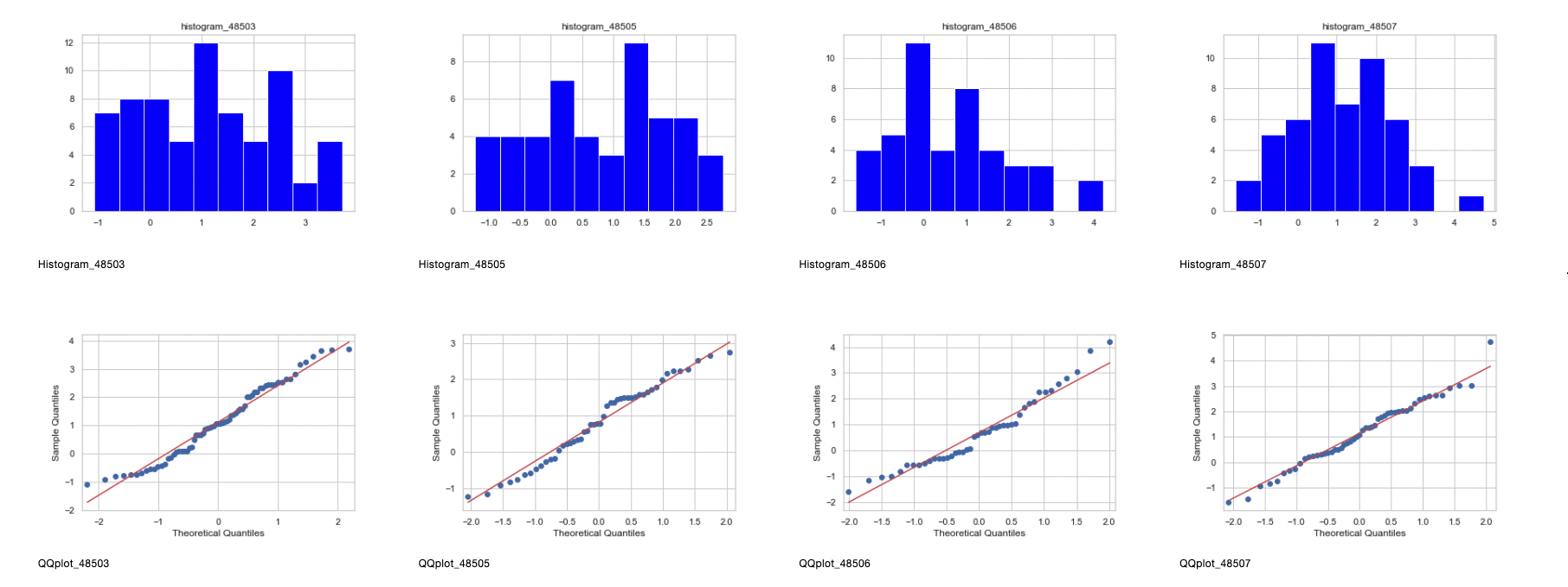
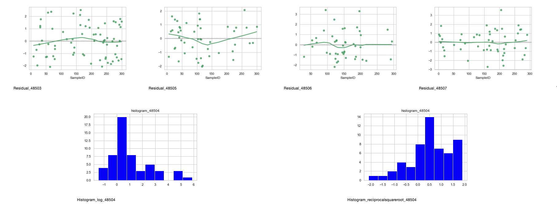
- Zip codes 48505, 48506, and 48507 definitely show normality after transformation from the histograms, QQplots, and residuals.
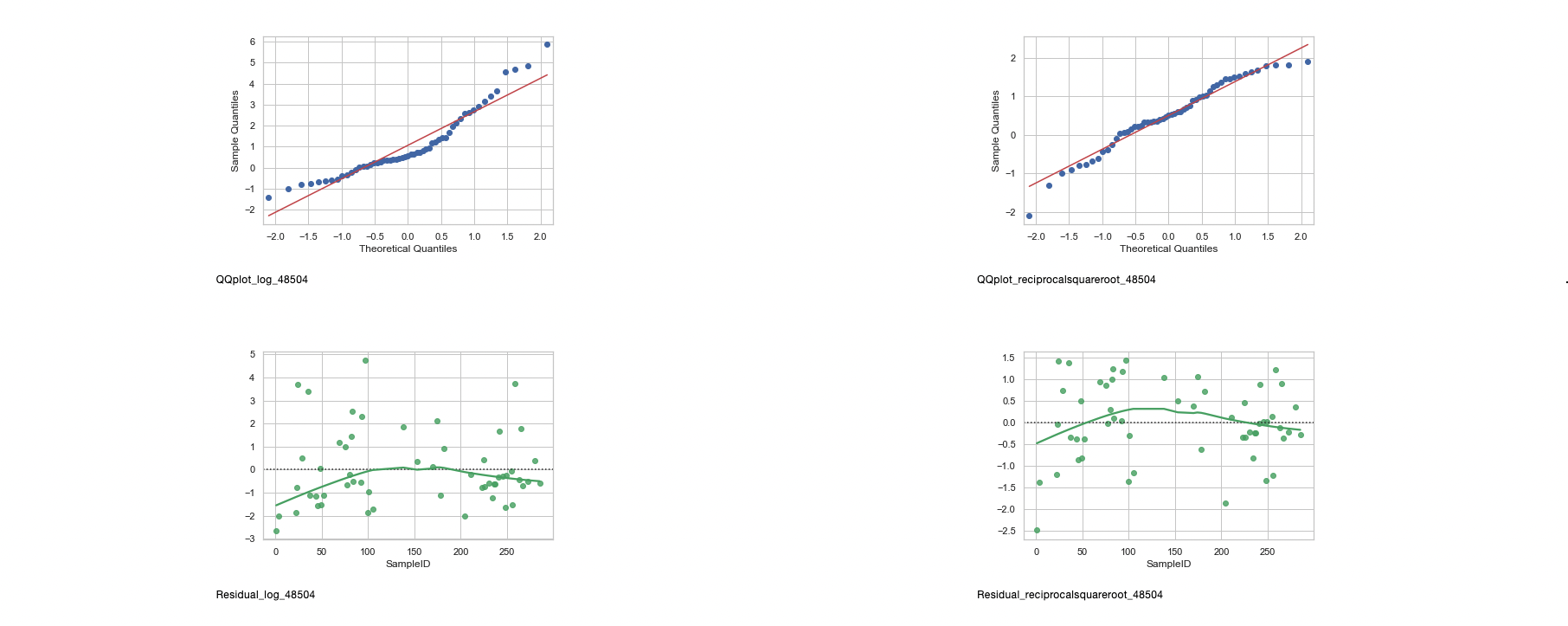
- Zip code 48504 shows normalcy when it comes to the reciprocal square root transformation, however, since the 2-Sample T-Test and ANOVA are parametric, 48504 will be removed from the analysis, leaving zip codes 48505, 48506, and 48507.
- 48503 will be considered as the p-values for the two failed normality tests are close to 0.05.
        ### 2-SAMPLE T-TEST ###

        ## Levene Test for Equality of Variances
        f_value, p_value = stats.levene(zip48505, zip48507, center = 'mean')
        lev = "LEVENE, f-statistic = {} and the p-value = {}".format(f_value, p_value)

        RESULT:
        LEVENE, f-statistic = 0.953888100345899 and the p-value = 0.3311610901946488


        ## 2-Sample T-Test
        f_value, p_value = stats.ttest_ind(zip48505, zip48507, equal_var = True)
        tte = "T-TEST, f-statistic = {} and the p-value = {}".format(f_value, p_value)

        RESULT:
        T-TEST, f-statistic = -1.3088359267078675 and the p-value = 0.19368231349358914
- The average lead content of the least contaminated zip code - 48505, is NOT statistically less than the lead content of the most contaminated zip code - 48507.
            ### ANOVA ###
            zip48503 = stats.boxcox(df_zip.loc[df_zip['Zip Code'] == 48503, 'Mean'], 0)
            zip48505 = stats.boxcox(df_zip.loc[df_zip['Zip Code'] == 48505, 'Mean'], 0)
            zip48506 = stats.boxcox(df_zip.loc[df_zip['Zip Code'] == 48506, 'Mean'], 0)
            zip48507 = stats.boxcox(df_zip.loc[df_zip['Zip Code'] == 48507, 'Mean'], 0)

            f_value, p_value = stats.f_oneway(
                    zip48503,
                    zip48505,
                    zip48506,
                    zip48507)

            aov = "ANOVA, f-statistic = {} and the p-value = {}".format(f_value, p_value)

            RESULT:
            ANOVA, f-statistic = 1.5599746050592251 and the p-value = 0.20021052741591835


            ### PAIR-WISE COMPARISON ###
            df_zip = df_zip.drop(df_zip[df_zip['Zip Code'] == 48502].index)
            df_zip = df_zip.drop(df_zip[df_zip['Zip Code'] == 48504].index)
            df_zip = df_zip.drop(df_zip[df_zip['Zip Code'] == 48529].index)
            df_zip = df_zip.drop(df_zip[df_zip['Zip Code'] == 48532].index)

            df_zip['Mean'] = stats.boxcox(df_zip['Mean'], 0)

            RESULT:
            Multiple Comparison of Means - Tukey HSD,FWER=0.05
            ============================================
            group1 group2 meandiff  lower  upper  reject
            --------------------------------------------
            48503  48505  -0.2964  -0.9132 0.3204 False
            48503  48506  -0.4314  -1.0645 0.2017 False
            48503  48507   0.0185  -0.5875 0.6245 False
            48505  48506   -0.135  -0.8199 0.5499 False
            48505  48507   0.3149   -0.345 0.9748 False
            48506  48507   0.4499  -0.2253 1.1251 False
            --------------------------------------------
- There is NO statistical difference between the means of the zip codes.
            ### KRUSKAL NON-PARAMETRIC TEST ###
            f_value, p_value = stats.kruskal(
                    df_zip.loc[df_zip['Zip Code'] == 48503, 'Mean'],
                    df_zip.loc[df_zip['Zip Code'] == 48504, 'Mean'],
                    df_zip.loc[df_zip['Zip Code'] == 48505, 'Mean'],
                    df_zip.loc[df_zip['Zip Code'] == 48506, 'Mean'],
                    df_zip.loc[df_zip['Zip Code'] == 48507, 'Mean'])

            kru = "KRUSKAL, f-statistic = {} and the p-value = {}".format(f_value, p_value)

            RESULT:
            KRUSKAL, f-statistic = 4.941524818598804 and the p-value = 0.29335021081060986
- Similarly, the Kruskal-Wallis H-test shows that there is NO statistical difference between the medians of non-transformed data.
-- END --
